Introduction
References and meta-references
What is binary morphology?
What about boundary conditions?
The rasterop implementation of
binary morphology
The destination word accumulation
implementation of binary morphology
Separable atomic operations, sequence interpreters and simplicity of use
Summary of available implementations
Binary morphology and cellular automata
Binary morphology is set of fundamental operations on binary images
(2-D sets of boolean values). It is a very simple, nonlinear
convolution-like operation
between two such sets. Unlike linear convolution, morphology
takes the Min and Max of elements in the set.
One set is the image per se; the other
is the kernel of the convolution, which is called a structuring
element and has a defined origin (sometimes called the
"center"). Binary morphology is extremely important for fast,
low-level image matching operations -- every commercial "machine vision"
system has it because of its usefulness. Back in the period around
1990, if you wanted to do fast pattern matching, you could buy
such a system from any one of several firms (see below). These implemented
binary morphological operations on custom systems with wide
registers at about 1 billion pixel operations/second. Today, using the
destination word accumulation method (implemented in Leptonica)
on a 1 GHz CPU, you can do binary morphology up to an order of
magnitude faster! So if you need fast matching operations on
binary images, read on. And if you are doing image analysis on grayscale
or color images, binary morphology can often be used to give quick and
spatially detailed "answers" to questions of interest.
I recommend the following references for initiates and practitioners:
If you are familiar with morphological image processing, you can skip this section.
There are many fields, such as computational linguistics, materials science and biology, that use the term "morphological" to describe the objects they study. To distinguish itself from these, morphological image processing is sometimes called "image morphology" and "mathematical morphology," the latter perhaps to indicate the degree of abstractness that has been achieved. Image morphology was pioneered in France in the 1960s by Matheron and Serra, and further developed in Europe thereafter. But until the early 1990s, most image processing in the U.S. was linear: linear convolution and invertible transforms. Heavy mathematical machinery can be brought to bear on such linear processing, but there are many situations where non-linear image processing is required, especially in image analysis applications where decisions need to be made. (You can't make decisions with linear operations, which don't allow you to say "yes" or "no" -- only degrees of "maybe".) The neglect in the U.S. of these fundamental nonlinear operations reminds me of the old joke about someone who loses his keys at night but only searches for them under a lamp-post because "that's where the light is." I believe that the first doctoral thesis on image morphology in the U.S. was the 1985 work on nonlinear filters by Petros Maragos with Ron Schafer at Georgia Tech.
Around that time, several "machine vision" companies were founded in Michigan, largely to provide automated inspection for local auto manufacturers. Binary morphology was used as a principal technique because it is fast, memory efficient and provides general routines for pattern matching. These companies sold special purpose hardware because it was lucrative and it was difficult to put the algorithms on general purpose machines. Why was that? After all, the Motorola 68020 was available in 1985 and the Intel 386 was available in 1986. Each of these supported memory-protected multiprocessing with 32 bit addressing. The main problem was that DOS and Intel lived in a 16 bit world, using a 64K segmented memory model, and it was difficult to handle larger images. And the unix workstations that were built around the 68020 were relatively expensive. They were also slow -- these chips ran at a few MHz, several hundred times slower than the ubiquitous 3 GHz chips you can buy for $100 today. These machine vision systems were also popular because they were designed to be special purpose "turn-key" systems (though it was not always easy to turn the key, especially when you programmed them in an assembly-like language.) And so, into the early '90s, there was a market for this special purpose hardware. But the inexorable progress of the basic PC microprocessor, both in speed and in software tools for program development, has greatly reduced the demand for these special systems -- just as Silicon Graphics found that its business with special purpose graphics hardware was obliterated by cheap, fast Intel and AMD chips with gigaflop graphics performance. Today, processors are fast, memory is cheap, and we can use binary morphology for pattern matching at speeds that were not imagined even 10 years ago.
Binary morphology is about operations on sets. The sets are ON (black) pixels in a 2-dimensional image. As with all image processing operations, there is a source image that is operated on to produce a destination image. In the following, we use one set of conventions to describe the erosion and dilation operations as set operations. Other conventions exist, and you should keep this in mind when you read the literature.
The basic binary morphology operations are dilation and erosion . In a binary image, we refer to the foreground (black) pixels variously as "black", "foreground", "ON" or "1". We refer to the background (white) pixels variously as "white", "background", "OFF" or "0". Loosely speaking, dilation "smears" the foreground and erosion "thins" the foreground. These two operations are actually dual in that an erosion of the foreground is equivalent to a dilation of the background. Dilation can be implemented as follows: start with a cleared destination image (all OFF pixels). Then do a sequence of logical OR operations of the source image with the destination, each time with a specific shift, as determined by a pattern called a structuring element (Sel). The Sel is a 2-dimensional pattern of hits, all relative to an origin that is often referred to as the center of the Sel. It is a set as well. So there are really two sets involved in a morphological operation: the image and a Sel. For example, consider a Sel that is a horizontal pattern of 5 contiguous hits (x,y) = {(-2,0), (-1,0), (0,0), (1,0) and (2,0)}, with an origin at (0,0). Then a dilation of the image by this Sel involves initializing all dest pixels to OFF and then ORing the source five times with source shifts given by the five hits in the Sel.
An erosion can be implemented in a similar way. For example, you can initialize all dest pixels to ON and then do a set of logical ANDs between the dest and the shifted source. But there is one important difference: you take the shift to be from the hit to the Sel origin, rather than from the origin to the hit. You can think of the Sel as a set of vectors in two dimensions, and for erosion, you use an inversion of these vectors. Because of the AND, you end up with ON pixels in the destination only where the hits of the Sel can all fit on the ON pixels of the source image. In fact, the erosion can be implemented by placing the Sel with its origin at every ON pixel in the source image and, for every location where all hits in the Sel are placed on ON pixels in the image, an ON pixel is produced in the destination at the location of the Sel origin. Thus, the erosion is a pattern matching operation. The inversion of the Sel for erosion is required to make the erosion a dual of the dilation. The prescription for erosion just given is oversimplified; see the discussion in the next section on boundary conditions.
The inversion of the Sel for erosion is also required to make the opening, which is a sequence of erosion followed by dilation, both using the same Sel, have the property called idempotence. This means that if you do a second opening, there is no change after the first one. Operations that are idempotent have a special significance. The opening can be visualized as follows: it gives you only those ON pixels where the Sel is able to fit entirely in the foreground. (The erosion gave on pixels only at the Sel origin location of such a pattern match. Then by dilating those pixels, with the same Sel, you get all the pixels in the match.) So the opening projects out a subset of pixels of the source image, and a second opening gives the same result because the Sel fits in those pixels by construction. The closing, which is a dilation followed by an erosion with the same Sel, is also idempotent. It is the dual to the opening, because you can do a closing by opening the background. Regardless of the convention that is used to define erosion and dilation, the opening and closing operations have a unique definition. All four morphological operations have two important properties:
Unlike dilation and erosion, the result of opening or closing an image does not depend on the location of the origin of the Sel. (This is another reason for inverting the Sel for erosion.) A consequence of this is that opening and closing have special properties besides idempotence not shared by erosion and dilation. Namely, the opening is anti-extensive, which means that the set of ON pixels after opening is contained in the source image. Oppositely, the closing is extensive because the source image ON pixels are all contained in the image that results from closing it. The erosion and dilation do not have these properties because the result depends on the location of the Sel origin. For example, if you dilate an image with a Sel that has a single hit offset from the Sel origin, the result is simply a translation of the original image by the vector from the Sel origin to that hit. For this case, are the ON source pixels all contained in the ON pixels of the destination?
You might think that all important operations are translationally invariant, but this is not true. For example, any operation that scales the image size is not translationally invariant. For example, if an image is reduced by subsampling, the resulting image depends on the subsampling grid (i.e., on the specific pixels that are chosen to represent the reduced image). A translation of the image relative to this grid before subsampling can result in a different (translated) image from that produced by subsampling at the original grid location.
There is another important morphological operation, the hit-miss operation. It is a very general pattern match because it finds matches to parts of the image that have specified OFF pixels as well as ON pixels. For example, the lower edge of a horizontal line in the image can be found with a hit-miss Sel that has a row of misses below a row of hits. For a pixel to be set ON in the destination, all the hits must be on ON pixels and all the misses must be on OFF pixels in the source. (The operation is sometimes called ``hit-or-miss", but the operation is really a hit-and-miss.) Thus in its most general form, the Sel has in each location either a hit, a miss or a don't-care. The addition of misses to the Sel makes the hit-miss operation very useful, but it loses the increasing property. (Can you see why?). Consequently, it is not of great interest in set theory because without a preservation of image ordering, relatively few general statements can be made.
I should not leave you with the impression that this is
all there is to binary morphology. There are many other
image operations, such as thinning (with or without
preservation of connectivity), that can be formed
by sequences of basic operations. There are also many
nonlinear transforms from binary to grayscale images,
such as a simple distance transform that labels the minimum
distance from each pixel to a pixel of opposite color.
A more complicated nonlinear function
labels connected components (a set of pixels of the same
color for which each pixel in the set is adjacent, in either a 4- or
8-connected orientation, to another pixel in the set) by computing
a measure of their "length" as the maximum, over all
pairs of pixels in the set, of the minimum
distance between the two pixels, taken over all paths
between them that stay entirely within the set of pixels
that constitute the connected component.
Further, all the binary morphological
operations can be generalized to grayscale, where the
dilation is a Max operation and erosion is a Min
operation. (Do you see how the binary dilation and erosion
are a special case of taking the Max and Min
operation? With a binary image, the max value is 1 and
the min value is 0. An erosion places a value of 0 at the Sel
origin unless all the pixels under the Sel are 1. Therefore,
the erosion selects the minimum of the binary pixel values.)
And once you go to grayscale, the number of
interesting nonlinear operations explodes. For example, much
work has been done on image segmentation, typically using
seeds and region growing. See the literature for details.
What is the mathematically elegant definition? It is the one that treats erosion and dilation as duals, even in the presence of boundaries. We will call it the symmetric boundary condition (SBC): extend an image by the min value (0 for binary images) for dilation and by the max value (1 for binary images) for erosion. This gives strict duality. To avoid confusion, we call the extra pixels that are used to extend the image beyond its actual boundaries the frame pixels.
However, for document images, there is a natural bias toward extending the image with background (0, OFF) pixels, for both dilation and erosion, because we typically have background pixels at the boundaries. So we might want to handle the boundary conditions by requiring that we get the same result as if the image were actually extended sufficiently by 0 pixels, for all morphological operations. This does not give strict duality between dilation and erosion, but I find it preferable for document imaging applications. We will call this the asymmetric boundary condition (ABC).
Erosion is thus different for SBC and ABC. Suppose you have a binary image with all pixels ON. An erosion with a 3x3 Sel flips a 1 pixel wide border around the image to OFF using ABC, and has no effect on the image using SBC.
The most problematic operation on document images is closing. Consider a document imaging application with binary images, and let's take a specific closing example. Suppose you have an image with one ON pixel, located near the left hand edge at (x=5,y=50), in an image of size 100 x 100, and you dilate with a horizontal structuring element of width 21 pixels with the origin at its center. Here are the three cases:
In Leptonica, you get to choose which convention -- ABC or SBC -- you want to use. There is a function, resetMorphBoundaryCondition(), that takes one of two values, SYMMETRIC_MORPH_BC and ASYMMETRIC_MORPH_BC. We initialize it to ABC, so that by default all pixels outside the image are assumed to be 0 (OFF) for both dilation and erosion. The disadvantages of this convention are that we lose duality near the boundary, and have to be careful with closing. However, we gain the condition that an erosion cannot bring ON pixels in from the boundary onto an image that is mostly OFF near the boundary, as most binary document image pages are. If you do a translation (which could be implemented as either a dilation or an erosion by a Sel with one hit that is not at the Sel center), and you don't want to introduce a rectangle of black pixels, you must use the convention that the image is surrounded by OFF pixels. If you use SBC with such a translation, you will introduce a rectangle of ON pixels in an erosion but not in a dilation.
As you can see, the type of boundary conditions you want to use may depend on your application. Most mathematicians would likely argue for using SBC. However, these issues are introduced here because SBC is not the only possible choice, and with Leptonica you can decide which boundary conditions you want to use.
We discuss below exactly how we handle the boundary conditions.
It turns out that there is essentially no difference in implementation
complexity or efficiency between the two choices, for either
of the two implementations we give here. Those implementations
are discussed below: full-page rasterops and destination
word accumulation.
As described in the previous section, a morphological operation can be implemented by performing a sequence of logical ORs (for the dilation) or logical ANDs (for the erosion) of the source image, translated each time according to one of the hits in the Sel. The rasterop can be used, where the rectangle chosen is the entire source image. For all rasterops, the source image is clipped so that it does not try to write beyond any edge of the destination. There are other details, of course, such as the initial conditions on the destination image and the handling of the boundary conditions.
We have already introduced the issue of different conventions for choosing boundary conditions for erosion. We can imagine implementing erosion by rasterops in two ways:
We use the second method because of its simplicity, and because it can be used directly to implement erosion with both SBC and ABC.
Now, when an image is shifted to the right by 2 pixels, the leftmost 2 columns of pixels in the destination are unaffected by the AND. What should happen to these 2 columns? It depends on whether you are using SBC, which logically brings in ON pixels from the frame, or ABC, which logically brings in OFF pixels from the frame. (But if we do full image rasterops without a frame, nothing is actually brought in -- the 2 columns of pixels are simply not altered.) If you are using SBC and initialize the image pixels to ON, these 2 columns remain ON, just as if you really pulled ON pixels in from the frame. If you are using ABC, regardless of image content you must clear these columns out later.
Suppose we are using asymmetric boundary conditions, where we require that the result of erosion using rasterops is equivalent to a situation where the source is surrounded by enough OFF pixels to cover the dest for every translation specified by the Sel. Details on this choice of boundary condition convention can be found in a recent paper on the Implementation Efficiency of Binary Morphology . We have two methods for insuring that the pixels near the boundary are properly cleared. We can extend the source image with OFF pixels all around, and clip each rasterop to the destination image. Then those columns of OFF pixels would automatically clear the destination because of the AND operation. Or equivalently, without embedding the source image in a larger image of OFF pixels, we can perform all the rasterops in the erosion with usual clipping to the translated source image and, as a final step, clear the (up to) four rectangles of the appropriate boundary pixels in the destination. For each such rectangle, the size in a direction normal to the boundary is equal to the maximum shift (relative to the Sel origin) in the corresponding one of the four directions. For example, if the maximum shift to the right in the Sel is 4 pixels, the rectangle consisting of the 4 left-most columns of the destination must be cleared. (Remember that for erosion, the vector giving the image shift for each hit in the Sel is from the hit location to the Sel origin.)
We must also clear the edge pixels for the hit-miss transform, because it is a near relative of the erosion. The size of the rectangles to be cleared is determined from the hits in the Sel, exactly as in the erosion. The location of the misses in the Sel are not important for the clearing operation because the pixels that would be brought in from beyond the image boundary (if it were extended) would be ON. This is because for each miss, a translated version of the negative image is ANDed.
Suppose on the contrary that you wish to adopt the symmetric boundary conditions; namely, that the image is surrounded with ON pixels for an erosion, as discussed above. Then you simply use the second method for the erosion given above: set the dest image pixels (to 1); then AND each raster operation, properly shifted and clipped. This operation is dual to the dilation, and you stop there -- you don't clear the edge pixels. For closing, with the example given in the previous section, we do not need to add any surrounding frame pixels for the rasterop implementation. After the dilation, we set all destination pixels ON for the erosion and do the set of ANDs from the source (which is the destination of the previous dilation). Because of rasterop clipping, it's easy to see that the line of pixels from the original to the left boundary will be preserved by the erosion.
As mentioned in the previous section, you can determine the boundary conditions using the function resetMorphBoundaryCondition(). The effects of the boundary are most striking with the closing operation. Closing is formally extensive, but with the ABC convention without added frame pixels, ON pixels near the image boundary can be removed because the dilation does not extend past the boundary. If you are using the ABC convention, the function pixCloseSafe() will remove this anomaly by adding a frame of minimal required size to every image before closing, and removing the frame pixels at the end. The routines for adding and removing a such a frame are in pix2.c. (In the libarary, we refer to this as adding or removing a border). Note again that if you are using SBC, closing will be extensive without the addition of actual pixels around the boundary, and the anomaly will be avoided automatically.
The source code for the rasterop implementation of binary morphology is in morph.c. A few things to note are:
PIX * pixDilate(PIX *pixd, PIX *pixs, SEL *se);The first argument is the dest; if it is NULL, a new dest pix is allocated. The function returns the dest in all circumstances. If pixs and pixd are pointers to the same Pix, the operation is in-place, and pixs will be changed; otherwise, pixs is unaltered.
To avoid writing special case functions for words that are at or near the image boundaries, dwa is implemented on interior pixels that are more than 32 pixels from the actual image boundary. The outermost 32 pixel border of pixels within the image are read from but not written to. If in an application it is desired to operate on all pixels in the image, the user must add a border of frame pixels before doing a dwa dilation or erosion. It is also necessary to add the frame pixels with the correct initial color. For dilation, the pixels added to the destination are always 0 (OFF). For erosion, they are OFF for ABC and ON for SBC. This could be automated if the pix had a field specifying the frame size, but I felt that adding this much machinery to slightly simplify the use of dwa morphology was not warranted. Just keep in mind that dwa usage requires a border of extra frame pixels if you don't want to get get boundary artifacts, and you must initialize the pixels properly according to the convention you are using.
            PIX * pixMorphDwa_1(PIX *pixd, PIX *pixs, INT32 operation, char *selname);
            PIX * pixFMorphopGen_1(PIX *pixd, PIX *pixs, INT32 operation, char *selname);
The use of the first two arguments is standard, as described
above for the rasterop implementation. The operation is
one of the set {L_MORPH_DILATE, L_MORPH_ERODE,
L_MORPH_OPEN, L_MORPH_CLOSE}, and the
Sel to be used is specified by the
name string (the selname) associated with that Sel.
The list of allowed name strings for the Sela
is automatically extracted and placed in the file
fmorphgen.1.c.
            PIX * pixHMTDwa_1(PIX *pixd, PIX *pixs, char *selname);
            PIX * pixFHMTGen_1(PIX *pixd, PIX *pixs, char *selname);
The code generated by fhmtautogen() with index = 1
is in files fhmtgen.1.c and fhmtgenlow.1.c,
and has been put in the library.
The only restriction beyond size on the hit-miss Sels
is that each one must have at least one hit; otherwise, the
code generated aborts with an error message.
With all the mechanisms set up for doing binary morphology with both rasterop and dwa, and for doing grayscale morphology, it is important to add some machinery to make it very easy to use for the situation where the Sels are linear operators of all HITS, which is by far the most common usage. These linear operators can be used in "separable" combinations, horizontal and vertical, to implement morphology with 2-dimensional rectangular Sels of all HITS. We call these 2-dimensional Sels "bricks." Large linear Sels, of which the bricks are composed, can themselves be decomposed for efficiency, and we do this with 2-way composites, giving a computation savings for a linear Sel of length n of about a factor of n / (2 * sqrt(n)) over the unary method without decomposition.
The machinery has two levels that are convenient for use: a lower level where the brick Sel morphologyical operations are directly invoked, and a higher level that is an interpreter to run a sequence of such operations. Specifically,
There are five sets of atomic functions for brick Sels, all with similar interfaces:
These all take the sizes of the horizontal and vertical dimensions of the structuring element, and do separable implementions when both dimensions are greater than 1. They are useful in their own right because they implement correct boundary conditions, including safe closing if chosen. They also handle all intermediate images transparently, of which there are several for separable openings and closings. And they don't require the generation and destruction of Sels, as they make them internally and destroy them after use. See the notes at the beginning of morph.c for usage.
For the operations using 2-way composable Sels, consider pixOpenCompBrick() as an example. The results are identical to to the those of pixOpenBrick(), for sizes that are exactly decomposed such that the product of factors in the former equals the Sel size of the latter. We place constraints and penalties on the functions that choose how to do the decomposition. The regression test prog/binmorph2_reg.c demonstrates the result of decomposition. For large Sels, the pix*CompBrick() functions are much more efficient. prog/binmorph2_reg also tests the dwa composable Sel operations, such as pixOpenCompBrickDwa().
The dwa brick morphological operations work on the set of linear Sels that are generated by selaAddBasic(), and which are implemented in dwa by the functions in fmorphgen.1.c. Look there to see which are available. If for some reason you want some other Sel, such as sel_23h, which is not there, you can follow one of the prescriptions set out in morphdwa.c. However, you will likely find that you don't need to do this, because the dwa operations that use 2-way composable Sels will implement a close approximation to sel_23h. For convenience, if you call the non-composite dwa version, such as pixCloseBrickDwa(), and the Sel doesn't exist for it, it will automatically call the 2-way composite dwa version, pixCloseCompBrickDwa().
To make these atomic functions even simpler to use, we provide interpreters for sequences of morphological operations. For binary morphology, these sequences are combined with rank reductions and replicative expansion. All the interpreters are in morphseq.c. The morphological operations enabled by the sequences all use separable brick Sels. As with the atomic brick dwa functions, the interpreters reduce the complexity of using a dwa implementation to s single function invocation with a simple interface.
How do we test all this? A large regression test, prog/binmorph1_reg.c, tests all the binary brick operations, including the 2-way Sel decomposition, along with their interpreted sequences. Specifically, we test all morphological operations using:
A second regression test, prog/binmorph2_reg.c, compares the results of the 2-way composite separable brick implementations (both rasterop and dwa) against the unary brick implementations. A third regression test, prog/binmorph3_reg.c, compares rasterop brick (separable and non-separable) with various implementations of separable dwa bricks.
Our default boundary condition is asymmetric
(0 for both dilation and erosion), but you can toggle this
to test all functions with using the symmetric b.c. as well.
A summary might help describe all these different implementations, and how they are used. The top-level for all these is in morph.c (full image rasterops) and morphdwa.c (destination word accumulation -- dwa).
As you can see, much of the machinery is specifically targeted for brick Sels. The reason is that in most applications, the vast majority of morphological operations use brick Sels!
There are a set of 3 regression tests, prog/dwamorph*_reg.c, that show you how to generate and use new Sels. prog/dwamorph1_reg.c calls a function to generate all linear Sels (both horizontal and vertical) from lengths between 2 and 63. This is a lot of code to add to the library, so instead, it compiles and runs two other programs with the code linked in. These programs are:
There are several things to notice:
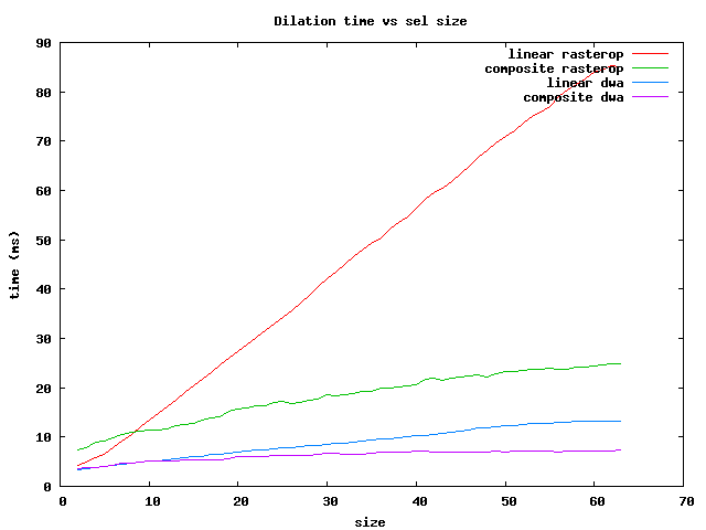
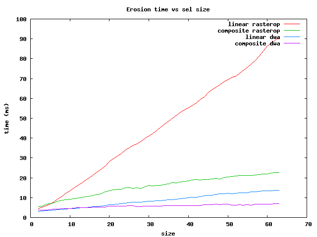
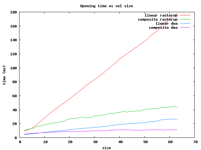
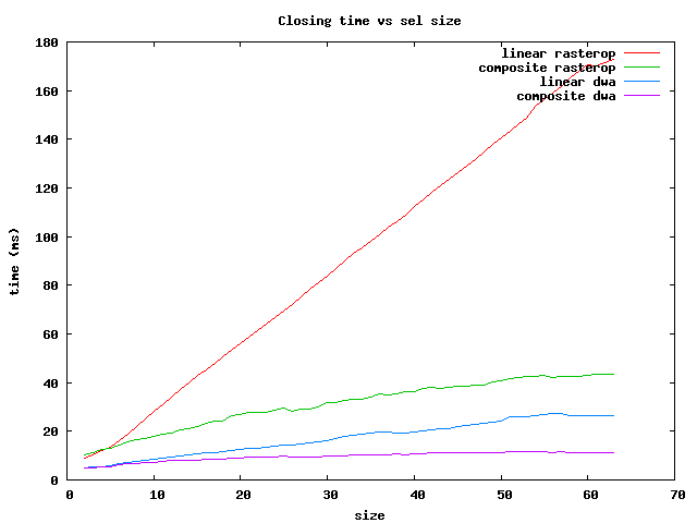
In summary, for the fastest operations on brick Sels, use the dwa composite
for sizes less than 64 and the rasterop composite for larger ones.
I can't leave this subject without mentioning cellular automata (CAs). Conway's "Game of Life" is an example of a cellular automaton (CA). In each generation (or iteration), a set of rules is applied to a binary image to generate another image. Conway used a very simple set of rules, where the value of a pixel on the next iteration depends only on the number of ON pixels adjacent to it. Too few neighboring ON pixels (starvation) or too many (overpopulation) caused the pixel to be OFF (die) in the next iteration. The result was a complicated and unexpected evolution of patterns.
Now I find it interesting that people only seem to use 2-D CAs. Not much happens in 1-D. Using a 3-neighborhood consisting of the binary pixel and its two neighbors in 1-D, you can have 23 = 8 different patterns, each of which can have a rule that sets the new pixel value to either ON or OFF. Thus, you can have 28 = 256 different sets of rules for how each pixel changes in the next iteration. A large number, but certainly manageable. But in 2-D, if your rule depends on the 3-neighbors, you can have 29 = 512 different patterns, leading to 2512 different sets of rules. That's a very large set, much too large to be usefully explored at random. With such large numbers, it is easy to see that people might be impressed with the computational power. And the numbers continue to explode in higher dimensions. For example, in 3-D, with a 3-neighborhood you have 227 patterns, and approximately 2130000000 different rule sets! I haven't seen anything done in 3-D, though I imagine it would be much more interesting than 2-D, though much harder to show visually what is happening.
For amusement, you can see some interesting 2-D CA at this web site. Each CA is described by its rule, which enumerates the output pixel result for each possible combination of neighbor pixels.
There is a simple relation between 2-D CAs and binary morphology. The hit-miss operation is a rule that gives a single pattern of ON and OFF pixels to be matched at each location, with the result that if the pattern is matched the output value is ON, and otherwise it is OFF. Any cellular automaton can thus be built as a generalization of the hit-miss operation, where in general more than one pattern is checked for a match. So in computational power, the hit-miss operation (thus generalized) is equivalent to the cellular automaton!
Things get even more interesting. Alan Turing's fundamental discovery was that all programmed computers are equivalent to a very simple Turing Machine that could read and write binary data on an infinitely long tape. Any machine that is equivalent to a Turing Machine is called Turing complete. And it is easily shown that cellular automata are Turing complete. Consequently, the hit-miss operator can be used to implement a Turing Machine! In principle, you can compute anything with this generalized hit-miss operator!
People who have spent a lot of time with CAs tend to become captivated by their power. I believe it is because the 2-D CA have both general computational power and, at the same time, are able to show us the computational evolution directly through our visual system, rather than analytically in some abstract mathematical representation.
The laws of physics can be expressed in many ways; among them, a local description of fields and their derivatives being the most common. The fields, which can be related to physical measurements, are the solutions to partial differential equations. These are solved on digital computers, typically by discretizing space onto a lattice and time into discrete increments, as a set of difference equations. A very simple example is the Laplace equation for the electrostatic potential in some region surrounded by a closed boundary on which the potential values are known everywhere. The solution on the lattice points inside is found by applying, over and over, a very simple rule: replace the value of the potential at each point by the average of the four closest neighboring values. This is a relaxation method; eventually the potential at each point arrives at its final value. You can implement this by a CA; for 2-D geometries, you can even implement it on a spreadsheet! (You may be worried because the world -- and spreadsheet cells -- appear to be described by real numbers instead of binary numbers. We'll sweep this objection under the rug by noting that real numbers can be approximated to arbitrary precision by binary numbers, patterns of 0s and 1s.) Because the laws of nature seem to be expressible locally by such very simple rules, people naturally wonder if the entire universe is, at the root, one big CA with some very simple rules.
There are two areas of physics in particular that have proven to be very difficult to explain, and that have recently forced physicists to develop new fields of mathematics. One is elementary particles, where things are not understood at the very small scales and mathematical descriptions tend to blow up. The other is in the macroscopic regime where we have particle interactions (e.g., in fluids) leading to complex nonlinear behavior such as turbulence and associated chaotic dynamics. In both cases, people naturally search for a set of simple underlying rules to explain the complex behavior. In particle physics, Wheeler speaks of the "quantum foam" at the scale of the Planck length, about 10-33 cm, where space-time itself is strongly perturbed by quantum gravity. Can rules at that tiny scale, perhaps given by a CA on a lattice, lead to the observed phenomenology of particle physics at much larger scales such as 10-17 cm? Likewise, people have observed chaotic behavior arising out of 2-D CAs, along with universal scaling parameters for the phenomena, such as period-doubling in chaos, that arise from very simple dynamical rules for the system evolution. So it is natural to hope that CAs can model and perhaps even explain the most difficult fields of physics. And why stop there? What about conscious intelligence, a mystery so slippery and deep that the mind is completely boggled at its contemplation? Could we possibly be CAs?
Edward Fredkin, a physicist at Boston University, has spent
much of his career on the search for the rules of the
universe based on the assumption that space and time are
discrete. A good introduction to his thinking is his 1992
paper,
A new cosmogony.
In 2002, Stephen Wolfram published his Opus Magnus,
A new kind of science, a 1200 page treatise on cellular
automata based on unpublished work he did over the past 10 years.
Wolfram, who got his PhD in physics from CalTech at age 20,
has a history of brilliant work, including founding the company
(of his name) that makes Mathematica. Like Julian Schwinger,
his motto could well be "If you can't join 'em, beat 'em,"
but unlike Schwinger, Wolfram is still in the game. I expect Wolfram
to make some important observations in this field.
