Image scaling is important for many situations in both image processing and image analysis. Consequently, a number of different scaling functions are provided in Leptonica.

Binary images at high resolution (300 to 400 ppi) can be used to make low resolution binary images for analysis or display on a low resolution device (such as a monitor). To make a version of a page image that is readable on a grayscale display, the scale-to-gray function can be used to produce a grayscale image (of at least 4 bpp) at about 100 ppi. Scale-to-gray can also be used to convert a binary image to a very low resolution grayscale page icon thumbnail at about 15 ppi. At such resolution, a 10 x 7 inch image shrinks to 150 x 105 pixels, which appears on a 100 ppi high resolution monitor as an icon of size 1.5 x 1.05 inches.

When scaling a grayscale or RGB color image, two things must be kept in mind. First, if the image is significantly reduced, it is useful to first apply a lowpass filter whose size is roughly the same as the subsampling factor, in order to reduce aliasing. Second, if the image is significantly enlarged, it is useful (though more expensive) to apply a linear interpolation to the original image, in order to avoid constructing blocks of equivalent pixels that are visibly "jagged" when simple pixel replication is used.

Finally, there is the upscale-to-binary operation, in which a grayscale image is upscaled to a higher resolution binary image. This is the inverse of scale-to-gray, and can be thought of as an example of image restoration; namely, restoring a higher resolution binary image, that had been previously downscaled to gray. We don't provide any estimation routines for this explicitly, but the operation can be performed with good results by a succession of two operations: grayscale upscaling using linear interpolation, followed by binarization using a threshold or dithering. (We provide several efficient composite operations of these types.)

Aliasing occurs when a signal is (sub)sampled at less than twice the wavelength of the highest frequency. To avoid aliasing, the high frequencies in the signal are removed with a lowpass filter before sampling. The sinc filter is ideal in that its representation in the fourier domain has constant value up to the cutoff frequency, where it goes to zero. Thus, it will remove aliasing with the smallest amount of blurring of the result. However, the sinc has infinite extension, and is impractical for efficient image processing. For our purposes, a reasonable compromise between acceptable blur and computational efficiency is to use a constant height convolution filter. The function pixBlockconv() has a computational time independent of the size of the filter, and is used for some of the lowpass filtering.

We enumerate and comment on these (four) operations in the next section, and then go into detail after that. See the table at the end of this page for an overview.

What types of image scaling are useful?

There are four main classes of image scaling:

1. grayscale --> grayscale
2. binary --> binary
3. binary --> grayscale (typically downscaling)
4. grayscale --> binary (typically upscaling)

How do you scale a grayscale image?

In the following, we are assuming that a scaling factor S is used, and that when S is larger than 1.0, the image is magnified (and the dest pixels are smaller than the source pixels), and when S is smaller than 1.0, the image is reduced (and the dest pixels are larger than the source pixels). In the actual implementations, we do not assume isotropic scaling, and provide two scaling factors: S_x and S_y.

Sampling.

The simplest scaling method uses sampling. If the image is reduced, we call it subsampling; if the image is enlarged it is replicative sampling. While this method is fast, it gives relatively poor results for both situations.

If the image is reduced, subsampling produces aliasing by the Nyquist theorem. Here's a simple illustration. Suppose the image consists of alternating light and dark pixel columns, and you subsample with a scale factor of 0.25. You are choosing pixels from every fourth pixel column. Every pixel you choose will be either light or dark, depending on where you start. The high frequency signal has entirely disappeared in the subsampled version. Now suppose the scale factor is 0.24, the first column you pick is dark, and you choose the column integer by truncating the floating point value. The second column you pick will be at 1/0.24 = 4.17 pixels, which is rounded to 4, so it will also be dark. The third will be at 8.33; rounded to 8 is a dark column. And so it continues, with the fourth at 12.5, the fifth at 16.67, and the sixth at 20.83, all dark columns. But the seventh, at 25, will be a light column. The next 5 columns will be also be light, until you get to the thirteenth, at 50.0, which is another dark column. Etc. You have a signal with a periodicity of 12 in the subsampled image. Nothing like this existed in the original. The low-frequency signal in the subsampled image, which corresponds to a periodicty of 50 pixels in the original, appeared through aliasing. To remove the aliasing, it is necessary to remove frequencies in the image whose periodicity is less than twice your sample spacing, because signals from those higher frequencies are aliased down into your reduced bandwidth. So here's the general rule to remove those high frequencies and avoid aliasing: Use a lowpass filter before subsampling.

If the image is enlarged by a large factor, pixel replication will give a blocky appearance. Each pixel will be magnified into a large block of pixels. Sharp edges will be enlarged, and lines that are nearly horizontal or vertical will have a stair-step appearance at their edges.

Area mapping (or area averaging) and lowpass filtering.

When an image is scaled, each dest pixel will partially or completely cover one or more source pixels. In area mapping, the dest pixel value is found by assigning it the average of the source pixels it corresponds to, weighting by the fractional area of each source pixel that it partially (or wholly) covers.

Strict area mapping is fairly expensive, compared to using a lowpass filter that averages entire pixels followed by downsampling. With large upscaling, it gives a result not significantly better than inexpensive replicative sampling. Consequently, it should only be used when downsampling. (Our rule of thumb is to use area mapping for downsampling with a scale factor less than 0.7). With very large downscaling (e.g., a factor less than 0.2), scaling by area mapping (pixScaleAreaMap()) does not give results much better than low-pass filtering followed by subsampling for antialiasing (pixScaleSmooth()). However, for scale factors between about 0.2 and 0.7, it gives significantly better visual results than pixScaleSmooth().

Let's consider scaling in more detail. Suppose you are enlarging the image, where the scaling factor is much larger than 1. Then most dest pixels cover just a small amount of a single source pixel. Relatively few dest pixels will overlap source pixel boundaries. In this case, the result of area mapping will be nearly identical to that of replicative sampling. Most dest pixels will be assigned the value of a single source pixel, so in this limit, area mapping reduces to subsampling except for the small number of dest pixels that lie across source pixel boundaries, where you get a weighted average of the source pixel values. The appearance, like the case for sampling alone, will be blocky, because you will see each source pixel magnified and with only a little fuzziness around the edge.

At the other limit, where you are doing a large reduction, each dest pixel covers many source pixels. If you take an average of the source pixels, including only the area of each source pixel that is actually covered by the dest pixel, you will get an unaliased and very good estimate of the value each subsampled pixel should have. However, doing this sum is computationally expensive, and the result is not appreciably better than simply doing an average (using an appropriate a lowpass filter) followed by subsampling.

As a good rule of thumb, for downscaling with a scale factor less than 0.7, you should use a lowpass filter and then subsample. To prevent aliasing, the size of the lowpass filter kernel on the source image should be approximately the area of the source that corresponds to a single pixel of the dest. The implementation of this approximate filter is straightforward; see pixScaleSmooth(). Better antialiased results are obtained by using strict area mapping, with a filter that is of constant (normalized) height over a rectangular region of the source image that corresponds closely to each dest pixel; see pixScaleAreaMap().

Mip-mapping.

Mip-mapping is the name given to the texture mapping method used in graphics (in particular, in games), where a multiresolution pyramid is constructed at power-of-2 scales, and each pixel at an intermediate scale is evaluated by interpolating between the corresponding pixels on the pyramid at resolutions above and below. It is widely used to display textures in graphics for two reasons: (1) the appearance of a texture (a set of neighboring pixels) varies smoothly as the resolution is changed, and (2) hardware to support the pyramids and perform the interpolations in real time is available in high-end graphics cards.

Mipmap scaling can be performed efficiently in the CPU, and we provide an implementation that is used in conjuction with scale-to-gray. For document images with text and sharp edges, mipmap scaling suffers from severe aliasing and should not be used if the quality of the images is important.

Min-max

Morphological transforms are the most important class of non-linear image transforms. Grayscale morphology, even using the van Herk/Gil-Werman method, is relatively expensive if you just want the min or max for each tile in a subsampled image. Rather than performing grayscale morphology on the full resolution image and throwing most of the results away with subsampling, for integer reduction it makes more sense to identify the tiles in the src image that correspond to each dest pixel and compute the min or max (for erosion or dilation) directly.

The function pixScaleGrayMinMax() performs this function for arbitrary (isotropic) downscaling. The speed is about 70 MPix/sec/GHz of source data. For the special case of downscaling by 2x, the function pixScaleGrayMinMax2() is about twice as fast again.

Min-max is a special case of the general rank order downscaler. The problem with the general rank order downscalers is that, except for the min and max values, they require sorting of pixel values. This is relatively expensive: sorting n elements is computationally of order n*log(n). For a 2x2 kernel (which we use here for filtering before a 2x reduction), this isn't too expensive. A general 2x rank order function pixScaleGrayRank2() allows a choice of the two intermediate rank values in addition to the min and max, but at about 3x the computational cost. For grayscale rank reductions greater than 2x, a sequence of 2x reductions with different ranks can be used to approximate an intermediate rank over the entire (power-of-2) reduction.

Linear interpolation

We describe the implementation(s) of linear interpolation in some detail because it is useful and conceptually simple, and because there exist very efficient implementations for the special cases of 2x and 4x upscaling. The general scaling implementations for linear interpolation of grayscale and RGB images are in the functions pixScaleGrayLI() and pixScaleColorLI(), respectively. They are appropriate for upscaling with a scale factor larger than 1, or for downscaling with a scale factor larger than about 0.7. For scale factors between 0.7 and 2.0, better results are achieved, particularly on orthographically generated images (as opposed to natural scenes) by a small amount of sharpening after scaling.

Implementation of linear interpolation scaling

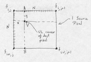
    A = (1/N) [(N - x)fi,j + xfi,j+1]

    B = (1/N) [(N - x)fi+1,j + xfi+1,j+1]

    V = (1/N) [(N - y)A + yB]

      = (1/N2) [(N - x)(N - y)fi,j + x(N - y)fi,j+1 + y(N - x)fi+1,j + xyfi+1,j+1]

This is the normalized result. We choose N = 16 for convenience and sufficient accuracy. It is interesting to compare this to the formula for area mapping at constant scale, used in the rotation algorithm. The filters are identical!

Considerations of efficiency for linear interpolation scaling

The linear interpolation scaling of RGB color images is trivially implemented by pulling out each color component as an image, scaling it as described above, and combining the three scaled color images. However, this suffers from several sources of inefficiency, the biggest of which is the byte-wise extraction and recomposition to form the separate component images. This also requires allocation of the temporary images, and a separate step where the scaled bytes in each component image are again extracted and recombined to form RGB color pixels.

A much better way, which is about 3x faster, is to do the operation whereby each dest RGB pixel is computed from the appropriate source pixels, using separate computations on each component, and extracting the components by shifts and masks. These word-based operations are enabled by our decision to order the RGB components with the MSB leftmost in the 32-bit word, so that we can shift and mask to access and set individual components, without regard for the endian-ness of the hardware. For example, you will see the general color linear interpolation scaling operation in scaleColorLILow() as a direct analog of the grayscale version scaleGrayLILow(), opened up to operate on each component.

For special cases such as 2x linear interpolation, the operations can be increased by a factor of more than 10 by unrolling the loop for each 2x2 set of dest pixels, caching two of the four src pixels for use in the next 2x2 block, and using a special case for the last row of src pixels, where interpolation can only be done horizontally. We implement a function to do a single line, so that it is relatively easy to combine linear interpolation scaling with binarization (either thresholding or dithering). You can see all the byte GETting and SETting for 2x LI in scaleGray2xLILineLow(). We also have a similar 4x LI function, scaleGray4xLILineLow().

These two unrollings -- color and destination blocks -- can be combined. To get efficient color 2x scaling with linear interpolation, we play the same trick as with the general case: take the grayscale 2x LI function and unroll it further to handle each of the color components, generating the destination pixels on the fly. It's all laid out in scaleColor2xLILineLow(). I haven't done the analogous unrolling for 4x color LI scaling; if you need it, the implementation is straightforward.

You can judge whether these efficiency hacks are worthwhile from the computational speed. Here are the times in seconds for four of the functions, on an 8 M RGB color image upscaled by 2x, so that there are 32 M RGB destination pixels (128 MB), using a 2.8 GHz P4 with enough memory to avoid disk paging:

general LI color	2.4 sec
general LI color using 3 x (general LI gray)	5.4 sec
2x LI color	0.18 sec
2x LI color using 3 x (2x LI gray)	0.7 sec

The salient efficiency results for LI scaling are: (1) it's important to code the color case up specially (and not use grayscale LI scaling on each component separately), (2) there are huge savings for special scaling factors like 2x for both color and gray, and (3) the extra work to do this is relatively small.

The other basic conditions on LI scaling are: (1) do not use for scale factors below 0.7 because of aliasing problems and (2) for scale factors below about 2.0, best results are obtained by following the LI with a small amount of sharpening. See pixScale() for a high-level implementation of scaling that selects the operations based on the scale factor.

The high-level call pixScale() dispatches general scaling to binary, grayscale or color procedures, depending on the depth of the PIX. All these general scaling functions have two scaling parameters, one for horizontal and one for vertical. Scaling is isotropic when these two factors are equal, and anisotropic otherwise.

Consider now binary scaling, and imagine that the scaling is isotropic. There are two cases: the scaling factor(s) can be either greater than 1 (upscaling) or less than 1 (downscaling). As mentioned above, with grayscale images one should use linear interpolation with upscaling, and for downscaling it's best to use a lowpass filter before subsampling. For binary images, we simply replicate pixels when upscaling. When downscaling binary images, there are three choices:

You have the choice of making a binary or a grayscale reduced image. In both cases, subsampling is required, and the methods described above for avoiding aliasing apply here as well. Namely, you should apply a lowpass filter before subsampling. There are many ways to do this, using either linear or nonlinear filters. But the net result will have a much poorer appearance if you make a binary reduced image. In fact, a page of 8 pt font, scanned binary at 300 ppi and reduced 4x to 75 ppi binary, will be essentially unreadable on a screen, regardless of the lowpass filter used. However, if you use a 4x scale-to-gray reduction filter, where each reduced dest pixel is taken to be the average of the 16 corresponding source pixels, the text will be readable, though difficult. (For such small type, you should use a 3x scale-to-gray reduction filter.)

The implementation of Nx scale-to-gray requires taking each NxN pixel block in the binary source and converting it to a single gray pixel with correct normalization. Consider N=4. The sum of the 16 binary source pixels can take on 17 different values, from 0 to 16. This range must be mapped to 255 to 0. The value inversion is due to the convention that a binary black pixel (value = 1) gets mapped to black (value = 0) in a grayscale image. (The gray values increase with the lightness of the pixel.)

So for each dest pixel, we use a table to find the sum of black pixels in the NxN corresponding source pixels, and then use another table to map that sum to the output grayscale value. The 4x scale-to-gray is very simple, because 8-bit lookup tables can be used to accumulate the sums in two adjacent dest pixels at simultaneously. For each possible set of 8 adjacent source pixels, the sums of the first and last 4 are packed separately in different bytes of the table word. These words are then summed for 4 adjacent source rows, giving the sums for the two dest pixels. The second lookup table is then used twice to convert each sum to the final 8 bpp dest pixel value. The 3x scale-to-gray is more complicated because the inner loop of an efficient implementation computes 8 dest pixels from 3 rows of 24 source pixels. There is some additional shifting and masking, but the basic algorithm is the same, and again requires two different lookup tables.

We provide high-level interfaces for the following integer reduction values for scale-to-gray: 2x, 3x, 4x, 8x and 16x, in scale.c. For images scanned at 300 ppi binary, 3x scale-to-gray generates a 100 ppi grayscale image, which is comfortable to read on most computer screens. Likewise, for images scanned at 400 ppi binary, 4x scale-to-gray produces a correspondingly readable image. As usual, the low-level functions, that only take array pointers, ints and floats, and do all the bit munging, are provided in scalelow.c.

Because of the importance of creating good downscaled grayscale renderings of high resolution binary images, we also provide a high-level interface for scaling of binary to gray with an arbitrary isotropic scale factor. The function is pixScaleToGray(), and the source code describes the approach in some detail. Here is a summary of the problem. Binary images have sharp edges, so they intrinsically have very high frequency content. To avoid aliasing, they must be low-pass filtered, which tends to blur the edges. How can we keep relatively crisp edges without aliasing? The trick is to do binary upscaling followed by a power-of-2 scale-to-gray, rather than doing a power-of-2 scale-to-gray followed by rescaling in grayscale. For larger reductions, where you don't end up with much detail, you can use binary downscaling before the scale-to-gray, to reduce the amount of computation. And for very large reductions, the scale-to-gray operation can be done first with little loss in quality of the result.

The general function is implemented with the goal of getting high quality reduced grayscale images with relatively little computation:

1. For scalefactors > 1/8, do binary upscaling before scale-to-gray.
2. For scalefactors between 1/16 and 1/8, do binary downscaling before scale-to-gray.
3. For scalefactors < 1/16, do scale-to-gray (16x) first, and then grayscale downscaling.

As mentioned above (Class 4), it is useful to convert a low resolution grayscale or color image to a higher resolution binary image for printing, as most printers have binary output at the pixel level. (They can print gray appearance by applying a halftone mask to the grayscale or color image.)

To achieve smooth results, this should be implemented using an interpolated grayscale scaling function that is followed by binarization. Further, to limit the amount of allocated memory, it is best not to generate the full higher resolution grayscale or color image, but instead, use a minimum-sized buffer from which the binary pixels are immediately produced. Such an implementation is quite tricky for arbitrary size expansion, but it is relatively simple for 2x and 4x expansions. Fortunately, these two handle many common requirements.

Binarization can be produced by thresholding, error diffusion dithering, or ordered dithering using a halftone cell. For images of text, thresholding is fine, but if there are gray image regions, the results are far better with some type of dithering. Further, depending on the printer, a gamma factor should be applied to the grayscale image before dithering an image area, and for typical write-black laser printers, a gamma factor of between 2.0 and 2.7 is typically used to lighten the resulting printed image.

We provide two integrated scale-to-binary operations, with 2x linear interpolated scaling followed by binarization, in scale.c. The upscaled grayscale image pixels are kept in a buffer of not more than 3 lines, and binarization is performed by either thresholding or error-diffusion dithering. Low-level functions are in binarizelow.c.

We also provide two integrated scale-to-binary operations, with 4x linear interpolated scaling followed by binarization. The upscaled grayscale image pixels are generated 4 lines at a time, for binarization by either thresholding or error-diffusion dithering. For thresholding, the buffer size is 4 lines, and for error-diffusion dithering the buffer size is 5 lines. The source is also in scale.c, with the lowest level functions in binarizelow.c.

We have implemented three of these very simple functions, the choice of which depend on the src and dest depth, all for isotropic integer reduction factors. For downscaling RGB to grayscale, use pixScaleRGBToGrayFast(). For downscaling RGB to binary, use pixScaleRGBToBinearyFast(). And for downscaling grayscale to binary, use pixScaleGrayToBinaryFast().

• scale.c and scalelow.c. These have arbitrary scaling (up or down) by nearest pixel sampling. For grayscale and color, you get three additional choices. You can use linear interpolation for upscaling and moderate downscaling; you can use area mapping for downscaling with a scale factor less than 0.7; and you can use lowpass filtering followed by subsampling for downscaling with a scale factor less than 0.7. There are fast functions for reducing both scale and bpp together. You can use downscale scale-to-gray, with special cases for 2x, 3x, 4x, 8x and 16x reduction, and upscale scale-to-binary, with special cases for 2x and 4x expansion. There is also rank downscaling for grayscale by factors of 2, as well as min and max grayscale reduction by integer factors.
• binreduce.c and binreducelow.c. There are two types of 2x reduction of binary images: subsampled and rank-filtered. We also provide a cascade of 2x rank-filtered reductions.
• binexpand.c and binexpandlow.c. These have fast power-of-2 expansion of binary images.
• binarizelow.c. This handles low-level thresholding and dithering that are an intrinsic part of 2x and 4x upscale gray-to-binary.

The high-level functions, and the types of images that they operate on, are given in the table below. The scaling "type" is one of the following:

• "interp": interpolating
• "interp*": interpolating on color and grayscale; sampling on binary
• "sampl": sampling without interpolation or lowpasss filtering
• "antialias": low-pass filtering followed by sampling
• "areamap": accurate summation of src subpixels for each dest pixel
• "minmax": takes the min or max of components within square set of src pixels
• "scaletogray": conversion of binary to lower resolution 8 bpp gray
• "rank": rank filtering before sampling, only on 2x binary and gray reduction
• "replicate": replicative expansion, by integer factors

We give two tables. The first is for scaling operations that preserve the depth (except where a colormap exists and is removed).

  Name                     src depth w/o cmap   depth w/ cmap   type          scale factor
  ==========================================================================================
  pixScale                 1, 2, 4, 8, 16, 32   2, 4, 8         interp*       arbitrary
  pixScaleLI               2, 4, 8, 32          2, 4, 8         interp        arbitrary
  pixScaleColorLI          32                   -               interp        arbitrary
  pixScaleColor2xLI        32                   -               interp        2x expansion
  pixScaleColor4xLI        32                   -               interp        4x expansion
  pixScaleGrayLI           8                    -               interp        arbitrary
  pixScaleGray2xLI         8                    -               interp        2x expansion
  pixScaleGray4xLI         8                    -               interp        4x expansion
  pixScaleBySampling       1, 8, 16, 32         2, 4, 8         sampl         arbitrary
  pixScaleSmooth           2, 4, 8, 32          2, 4, 8         antialias     less than 0.7
  pixScaleAreaMap          2, 4, 8, 32          2, 4, 8         areamap       less than 0.7
  pixScaleAreaMap2         2, 4, 8, 32          2, 4, 8         areamap       2x reduction 
  pixScaleBinary           1                    -               sampl         arbitrary
  pixScaleGrayMinMax       8                    -               minmax        integer reduction
  pixScaleGrayMinMax2      8                    -               minmax        2x reduction
  pixScaleGrayRank2        8                    -               rank          2x reduction
  pixScaleGrayRankCascade  8                    -               rank          up to four 2x reductions
  pixReduceBinary2         1                    -               sampl         2x reduction
  pixReduceRankBinary2     1                    -               rank          2x reduction
  pixReduceRankBinaryCascade 1                  -               rank          up to four 2x reductions
  pixExpandReplicate       1, 2, 4, 8, 16, 32   2, 4, 8         replicate     integer expansion
  pixExpandBinary2         1                    -               replicate     power-of-2 expansion
  ==============================================================================================
                 Table of high-level depth-preserving scaling functions

The second table is for scaling operations that do not preserve the depth, such as downscaling binary to gray or upscaling gray to binary.

  Name                     src depth w/o cmap   dest depth    type          scale factor
  ==========================================================================================
  pixScaleRGBToGrayFast    32                   8             sampl         integer reduction 
  pixScaleRGBToBinaryFast  32                   1             sampl         integer reduction 
  pixScaleGrayToBinaryFast 32                   1             sampl         integer reduction 
  pixScaleRGBToGray2       32                   8             areamap       2x reduction
  pixScaleToGray           1                    8             scaletogray   less than 1.0
  pixScaleToGray2          1                    8             scaletogray   2x reduction
  pixScaleToGray3          1                    8             scaletogray   3x reduction
  pixScaleToGray4          1                    8             scaletogray   4x reduction
  pixScaleToGray8          1                    8             scaletogray   8x reduction
  pixScaleToGray16         1                    8             scaletogray   16x reduction
  pixScaleToGrayMipmap     1                    8             scaletogray   less than 1.0
  pixScaleGray2xLIThresh   8                    1             interp        2x expansion
  pixScaleGray2xLIDither   8                    1             interp        2x expansion
  pixScaleGray4xLIThresh   8                    1             interp        4x expansion
  pixScaleGray4xLIDither   8                    1             interp        4x expansion
  ==============================================================================================
             Table of high-level scaling functions that do not preserve depth

Several things should be noted about the tables:

• The depths of the source image that are supported by the operation are given both for images that do not have a colormap and for images that have one.
• Full RGB color images are stored with 32 bpp. We are, however, only using three 8 bit color components for RGB color (i.e., we ignore the A byte, which is typically used for blending two images).
• In the case of interpolative and area-map antialiased scaling on images with a colormap, the destination image depth is either 8 (gray) or 32 (RGB), depending on the colormap, which is removed.
• There is no redundancy in low-level implementations. For example, if the input image is binary, both pixScale() and pixScaleBySampling() call pixScaleBinary(), which calls scaleBinaryLow() to handle arbitrary scaling by sampling on binary images.