[Leptonica Home Page]
Color Segmentation
Updated: Aug 23, 2022
What is color segmentation and why do it?
There is an entire industry devoted to the problem of searching
images in a large collection of images. These are typically
images of scenes taken with a camera, rather than drawings
or other composed images. The query protocol for the search
is typically to choose some image and request "all images that
are similar." A related problem is to place each image in the
collection into a subset of similar images, doing some type
of unsupervised classification. These operations require
the ability to calculate a meaningful "distance" between two
images. Unsupervised classification follows a simple algorithm.
Given a distance function and a threshold, each image is
sequentially placed either into an existing class or
starts a new class, depending on the distance of that image
from the representatives of each existing class. The first
image to start each class is the representative for the class,
at least on the first iteration. There may be subsequent
iterations where the parameters of the classes are averaged
to find a "center" for each class in the parameter space.
How is the distance between images determined? That's
the hard part -- there's no obvious way. In fact, for two-dimensional
images, there are very few distance metrics (satisfying the
triangle inequality) that have been found. One of them is
the Hausdorff metric, which we use for classification of
binary shapes; e.g., see Jbig2 image compressing.
For color images, no useful metric distance is known.
IBM had a big R&D program called "Query By Image Content," or
QBIC for short. None of the published methods work
very well, so it continues to be an "interesting" problem to
academics. Image search works much better if there is some text
associated with the images: you do a text search and don't
bother about the pixels in the image. After an initial
fanfare, IBM seemed to give up on the QBIC project near the
end of the last century.
But if you wanted to write a QBIC program, what parameters
would you choose? Intuitively, you want to include both
color and shape information. Images of natural scenes usually
have many colors and complicated shapes. So the first logical
step would be to simplify both the colors and the shapes.
Once that is done, you still have the difficult problem of
finding a good way to use your simplified colors and shapes
to generate a meaningful "distance." The color segmentation
in Leptonica tackles the easy part: finding regions
of significant size and nearly uniform color. We offer it as
a starting point for any QBIC-like image search application.
There are other reasonable approaches this problem, notably involving
textures. Rather than smoothing out regions and looking for
a few representative colors, you can identify regular or irregular
patterns of colored shapes. Textures are sufficiently varied that
taxonomies are non-trivial and somewhat arbitrary. A possible
implementation would omit the smoothing step (described below),
and would select binary textures formed by assigning fg and bg to
two specific colors. For N colors, there are N(N-1)/2 color pairs,
and for small N (say, less than 8) a search of all pairs is
feasable. We won't pursue this any further here, but we do use
textures implicitly in morphological analysis of document images,
for segmentation.
How does color segmentation differ from color quantization?
The purpose of color quantization is to generate an approximation
to the original image with a smaller palette of colors.
If there is a relatively small number of colors, without a
high frequency pattern such as halftoning, such an image
will compress very well losslessly, often much better than
with lossy compression such as jpeg, where a fine-grained
set of RGB colors is used. In Leptonica we use octcube
partitioning and octree indexing because it allows fast
color quantization with arbitrary color accuracy. For
best accuracy, an octree that represents the most important
colors is combined with error-diffusion dithering to approximate
the original colors accurately in each small region of the image.
However, dithered images do not compress well losslessly.
In color segmentation, fidelity to the original image is not
a goal. Instead, you want a small set of regions, of
significant extent and with smooth boundaries, each of which is
of a uniform color, and with a relatively small total number of
colors in the image. We want the few resulting colors to
be the best representative of each subset of pixels. The result
is an image that has been "simplified," both in colors and
shapes. As will be shown, octcube indexing can be used to
accelerate some steps of the classification process.
Although it's not important for the application, color segmented
images have excellent lossless compression.
How do we generate the color segmented images?
The best description of the method used here is the code itself
(colorseg.c). The top-level function, pixColorSegment(),
has four parameters, of which two -- the smoothing parameter and
the number of final colors -- are the most important. The other
two parameters could be generated programmatically, but an argument
can be made to keep them for experimentation. One of these
parameters is the maximum number of colors to be quantized in
the first phase, and as a rough guide, this should be at least
twice the final number of colors. The other parameter is the
initial guess for the threshold euclidean distance for determining
if a color belongs to an existing class. This distance is
related to the radius of the resulting clusters, which is
related to the maximum number of clusters that will be found
in the RGB space. Guidelines are also given for the relation
between the input euclidean distance and the maximum number of
clusters.
The process has four phases:
- Greedy, unsupervised classification.
This is an iterative procedure. We start with the threshold
cluster radius and the maximum number of colors. Pixels are
taken in raster order. The first pixel becomes the representative
for the first cluster. Successive pixels are assigned to this
or other existing clusters, or become representatives for
new clusters. If the maxcolors limit is exceeded, the
threshold radius is increased by a multiplicative constant and
the process is repeated, until a cluster assignment is
made that obeys the maxcolors constraint. The average cluster
color is computed during accumulation.
- Reclassification using the cluster averages..
Each pixel is re-assigned to the cluster whose average color
is closest to the pixel color. This improves the assignment.
The cluster averages are stored in a colormap. We make the
time to compute the assignment independent of the number of
pixel clusters, by constructing an octcube in RGB space and
assigning to each cube the nearest color in the colormap.
Then for each pixel, we use table-lookup twice: first to find
the index of the containing octcube, and second to find the
nearest color in the colormap to that octcube. We also keep
track of the number of pixels assigned to each cluster.
- Smoothing regions and boundaries..
Starting with the color cluster with the most pixels, we
generate a binary mask where those pixels are fg and all other
pixels are bg. Then do a closing with a Sel size given
by the smoothing parameter. Xor the result with the initial
mask to find the new pixels to be assigned to this color,
and reassign them. Repeat for all colors.
- Reduce the number of colors to the input 'finalcolors'..
Identify all the pixels that are not in the most populated
color clusters, by building a binary mask over them.
Assign all these pixels temporarily to one of the color
clusters that will be saved. Then remove unused colors from
the colormap. This does a compression of the colormap,
causing a reassignment of the pixel values (which are just
the colormap indices). Finally, reassign all the pixels
under the mask to their closest color in the colormap.
We can use the same function from the second phase to do this,
except this time we only reassign the masked pixels.
How does a color segmented image look?
Here is a fairly busy image:
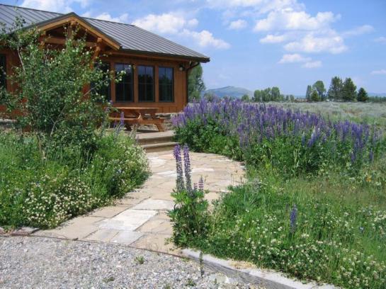
Suppose we want finalcolors = 4, and we use a 5x5 Sel for smoothing.
The rule-of-thumb says to choose maxcolors = 8 (approximately),
and we get:
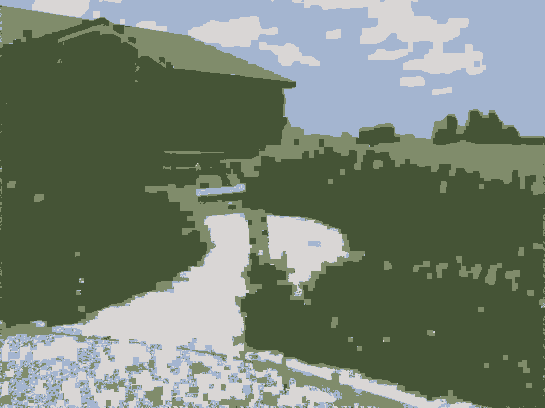
This isn't bad for using only four colors in the final result.
If we choose maxcolors = 4, the result is more random in the
final assignment:
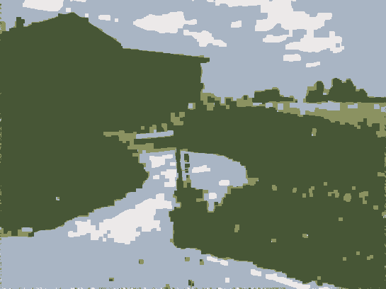
whereas going to the other extreme, starting with maxcolors = 16, the result
is very noisy:
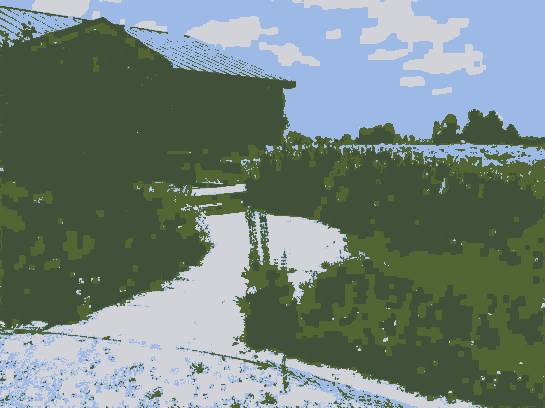
This is due to the fact that the smoothing step in
phase 3 was performed with many colors, and hence was relatively
ineffective. Then in phase 4, many of the pixels were reassigned
based on color rather than proximity. This suggests that we should
perhaps reduce the number of colors to the final value before
smoothing. I will leave it to the users of the library to
experiment further. Please let me know when you get some
interesting results, and I will post them here.
[Leptonica Home Page]

This documentation is licensed by Dan Bloomberg under a
Creative Commons
Attribution 3.0 United States License.
© Copyright 2001-2024, Leptonica